A half-wave rectifier is a rectifier that converts ac to dc and widely used for low-power applications. However, the practical application of this circuit is limited and worth studying in detail. Figures (i) and (ii) show the circuit and a voltage waveform of an uncontrolled half-wave rectifier with the resistive load that has a 240 V source of voltage at a frequency of 50 Hz with the load resistor 10 Ω.
First, determine the values of (a) the average load current, (b) the average load voltage, (c) the average load power, (d) the rms value of load current, (e) the rms value of load voltage (f) the rms value of load power and (g) the power factor of the circuit. After that, design the rectifier using Simulink MATLAB. Finally, compare the simulation result with the theory.
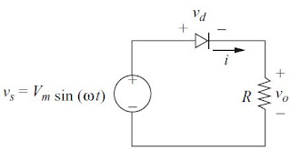 |
| (i) The circuit of uncontrolled half-wave rectifier with resistive (R) load |
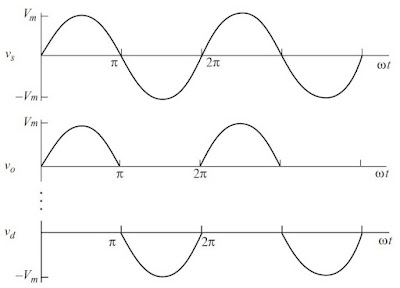 |
| (ii) The voltage waveform of uncontrolled half-wave rectifier with resistive (R) load |
List of symbols:
$I_{o,avg}$ average output current
$I_{o}$ output current
$I_{s,rms}$ source current in rms value
$I_{o,rms}$ output current in rms value
$V_{m}$ maximum voltage
$V_{d}$ diode voltage
$V_{o,avg}$ average output voltage
$V_{o}$ output voltage
$V_{s,rms}$ source voltage in rms value
$V_{o,rms}$ output voltage in rms value
$V_{f}$ forward voltage
$P_{o,avg}$ average output power
$P_{o}$ power output
$P_{o,rms}$ output power in rms value
$\omega $ angular frequency
$t$ time
$pf$ power factor
$R$ resistor
$S$ apparent power
Step 1: Theory
- The average load current, $I_{o,avg}$
\[I_{o,avg}= I_{o}= \frac{V_{o}}{R}=\frac{V_{m}}{\pi R}\]
\[V_{m}=\sqrt{2}\times V_{s,rms}\]
\[I_{o,avg}=\sqrt{2}\times 240\]
\[I_{o,avg}=10.80\:A\]
The average load voltage, $V_{o,avg}$
\[V_{o,avg}=V_{o}=I_{o}R=\frac{V_{m}}{\pi }\]
\[V_{o,avg}=\frac{\sqrt{2}\times 240}{\pi }\]
\[V_{o,avg}=108.04\:V\]
The average load power, $P_{o,avg}$
\[P_{o,avg}=P_{o}=P_{o,avg}I_{o,avg}=I_{o,avg}^{2}R=\frac{V_{o,avg}^{2}}{R}\]
\[P_{o,avg}=\frac{108.04^{2}}{10}\]
\[P_{o,avg}=1167.26\:W\]
- The rms value of load current, $I_{o,rms}$
\[I_{o,rms}=\frac{V_{o,rms}}{R}=\frac{V_{m}}{2R}\]
\[I_{o,rms}=\frac{\sqrt{2}\times 240}{2\times 10}\]
\[I_{o,rms}=16.97\:A\]
The rms value of load voltage, $V_{o,rms}$
\[V_{o,rms}=I_{o,rms}R=\frac{V_{m}}{2}\]
\[V_{o,rms}=\frac{\sqrt{2}\times 240}{2}\]
\[V_{o,rms}=169.71\:V\]
The rms value of load power, $P_{o,rms}$
\[P_{o,rms}=V_{o,rms}I_{o,rms}=I_{o,rms}^{2}R=\frac{V_{o,rms}^{2}}{R}\]
\[P_{o,rms}=\frac{169.71^{2}}{10}\]
\[P_{o,rms}=2880.15\:W\]
The power factor of the circuit, $pf$
\[pf=\frac{P_{o,rms}}{S}=\frac{P_{o,rms}}{V_{s,rms}I_{s,rms}}=\frac{V_{o,rms}}{V_{s,rms}}\]
\[I_{s,rms}=I_{o,rms}\]
\[pf=\frac{169.71}{240}\]
\[pf=0.707\]
Step 2: Simulation
For simulation, open the Simulink Library Browser and add blocks (Scope, AC Voltage Source, Diode, Series RLC Branch, RMS, Mean, Display, Voltage Measurement, Current Measurement, Goto, From, powergui, Product and Divide) to model.
Rearrange, copy and paste, and rename blocks accordingly, as shown in the figure below.
Click Series RLC Branch block and change the parameters to "Branch type:" to R, "Resistance (ohms):" to 10, and "Measurement" to None.
Click Diode block and change all the parameters to 0 and unclick Show measurement port.
Click Scope > File and set the Number of Input Ports > More... > Number of input ports: change to 4.
Click Mean blocks and change the parameter "Fundamental frequency (Hz):" to 50. Other parameters change to 0.
Click RMS blocks and change the parameters "Fundamental frequency (Hz):" to 50, "Initial RMS value:" to 240, "Sample time:" to 0, and click True RMS value.
- Click AC Voltage Source block and change the parameters "Peak amplitude (V):" to 240*sqrt(2), "Phase (deg:)" to 0, "Frequency (Hz):" to 50, "Sample time:" to 0 and "Measurement" to None.
- After setting all the parameters, change Stop Time to 2 and run the simulation.
- Click Scope block to shows the result of waveform $I_{o,rms}$, $V_{o,rms}$, $V_{s,rms}$, and $V_{d}$.
- Display shows the result of $I_{o,avg}$, $V_{o,avg}$, $P_{o,avg}$, $I_{o,rms}$, $V_{o,rms}$, $P_{o,rms}$, and $pf$.
Discussion
- The value of parameters for theory and simulation are almost equal.
- The waveform generated from the simulation is identical to the theory waveform.
Conclusion
The objection of this experiment is to compare the theory and simulation in terms of parameters value and waveform. The result shows that the value of the parameter of the theory is almost equal to simulation; the same goes for the waveform. Hence, the experiments were held successfully.
That all from me. If you have any suggestions, please write in the comment section. Thank you for your time 👷.


